Chapter 12 Cross-Validation
In creating statistical models, it is important to evaluate the performance of your model when deployed on new data.
Definition 12.1 Cross-validation is a statistical technique used to assess the performance and generalizability of a predictive model. It involves partitioning the dataset into multiple subsets, training the model on some of these subsets, and validating it on the remaining ones.
The goal is to evaluate how well the model will perform on unseen data and to reduce the risk of overfitting.
In this section, we will discuss some cross-validation methods to assess how good the model is in predicting a set of new observations.
There will be three cross-validation methods that will be discussed here:
- Validation Set Approach
- Leave-One-Out Cross-Validation (LOOCV)
- K-Fold Cross-Validation
All of these approaches involve calculating some evaluation metrics or cross-validation estimate. For an overview, here are some of them:
Regression
Let \(y_i\) be the actual observed value and let \(\hat{y}_{(i)}\) be the predicted value at level \(\text{x}_i\) using \(\hat{f}(\text{x}_i)\), where \(\hat{f}\) is a function that was estimated when the observation \(i\) was removed from the dataset.
The following are possible evaluation metrics in regression. Lower values are better.
- \(MSE = \frac{1}{n}\sum_{i=1}^n(y_i-\hat{y}_i)^2\)
- \(RMSE= \sqrt{\frac{1}{n}\sum_{i=1}^n(y_i-\hat{y}_i)^2}\)
- \(MAE=\frac{1}{n}\sum_{i=1}^n|y_i-\hat{y}_i|\)
- \(BIAS=\frac{1}{n}\sum_{i=1}^n(y_i-\hat{y}_i)\)
Classification
Suppose we are classifying \(y\) into two values (positive or negative). After modelling and predicting the classification of \(y\), we have the following confusion matrix.
| Predicted Positive | Predicted Negative | |
|---|---|---|
| Actual Positive | \(TP\) | \(FN\) |
| Actual Negative | \(FP\) | \(TN\) |
The following are some evaluation metrics for a binary classification problem. Higher values are better.
Accuracy: \(\frac{TP+TN}{TP + TN+FP+FN}\)
Positive Predictive Value (Precision): \(\frac{TP}{TP+FP}\)
Negative Predictive Value: \(\frac{TN}{TN+FN}\)
Sensitivity (Recall or True Positive Rate): \(\frac{TP}{TP + FN}\)
Specificity (True Negative Rate): \(\frac{TN}{TN+FP}\)
F1 Score: \(2\cdot\frac{Precision\cdot Recall}{Precision + Recall}\)
The choice of an evaluation metric will be based on the context of your data. All of these have functions in the Metrics package.
In this Chapter, we will focus on cross-validation of models that predict numeric variables, specifically with applications on multiple linear regression only.
12.1 Validation Set Approach
The train-and-test-set validation, or simply validation set approach, is a a very simple strategy for cross-validation.
The idea is to randomly split the set of observations into two parts, a training set and a test set (also called validation set, or hold-out set).
The model is fit on the training set, and the fitted model is used to predict the responses for the observations in the test set.
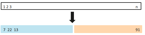
It is common to split the dataframe to 70-30: 70% of the dataset will be used for training the model, and the rest will be used for testing the model.
The resulting test set error rate is typically assessed using MSE or RMSE for quantitative response variables.
validation <- function(formula, data, size = 0.7, criterion){

    train_indices <- sample(1:nrow(data),
                            size = 0.7 * nrow(data))

    train_data <- data[train_indices, ]
    test_data  <- data[-train_indices, ]

    # Fit model on training data
    lm_fit <- lm(formula, data = train_data)

    # Predict on test data
    pred <- predict(lm_fit, newdata = test_data)

    # Extract the vector of observed y from test data
    obs  <- test_data[[all.vars(formula)[1]]]

    # compute and return evaluation metric
    eval <- criterion(obs, pred)
    return(eval)
}validation(income ~ urban, Anscombe, size = 0.7, Metrics::rmse)
validation(income ~ urban + education, Anscombe, size = 0.7, Metrics::rmse)
validation(income ~ urban + education + young, Anscombe, size = 0.7, Metrics::rmse)## [1] 552.6391
## [1] 368.039
## [1] 280.660812.2 Leave-One-Out Cross Validation
Leave-one-out cross-validation (LOOCV) is closely related to the validation set approach, but it attempts to address that method’s drawbacks.
Like the validation set approach, LOOCV involves splitting the set of observations into two parts. However, instead of creating two subsets of comparable size, a single observation \((x_1, y_1)\) is used for the validation set, and the remaining observations \({(x_2, y_2), . . . , (x_n, y_n)}\) make up the training set.
The processes is repeated for all observation to obtain \(n\) evaluation metrics, and their average will be obtained for an overall evaluation metric.
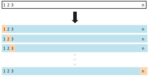
Procedure to estimate prediction error by leave-one-out cross validation
For \(k = 1, . . . , n\), let observation \((x_k, y_k)\) be the test point and use the remaining observations to fit the model.
Fit the model(s) using only the \(n − 1\) observations in the training set, \((x_i, y_i), i \neq k\).
Compute the predicted response \(\hat{y}=\hat{\beta_0} + \hat{\beta}_1x_k\) for the test point.
Compute the prediction error \(e_k = y_k − \hat{y}_k\).
Estimate the mean of the squared prediction errors \(\hat{\sigma^2}_\varepsilon=\frac{1}{n}\sum_{k=1}^ne_k^2\).
Most functions in R already show statistics from LOOCV approach (such as the PRESS), but we will demonstrate the LOOCV approach manually here.
loocv <- function(formula, data, criterion){
    n <- nrow(data)
    eval <- numeric(n)
    for(i in 1:n){
        train_i <- data[-i,]
        test_i  <- data[i,]
        mod_i   <- lm(formula,train_i)
        pred_i  <- predict(mod_i, test_i)

        y <- all.vars(formula)[1]
        eval[i] <- criterion(test_i[[y]], pred_i)
    }
    return(mean(eval))
}loocv(income ~ urban, Anscombe, Metrics::rmse)
loocv(income ~ urban + education, Anscombe, Metrics::rmse)## [1] 324.9626
## [1] 232.371212.3 k-Fold Cross-validation
An alternative to LOOCV is k-fold CV.
This approach involves randomly dividing the set of observations into \(k\) groups, or folds, of approximately equal size.
The first fold is treated as a validation set, and the method is fit on the remaining \(k − 1\) folds. This process results in \(k\) estimates of the evaluation metric. The k-fold cross validation estimate is computed as the average of the \(k\) metrics.
LOOCV is a special case of k-Fold CV, where \(k=n\).
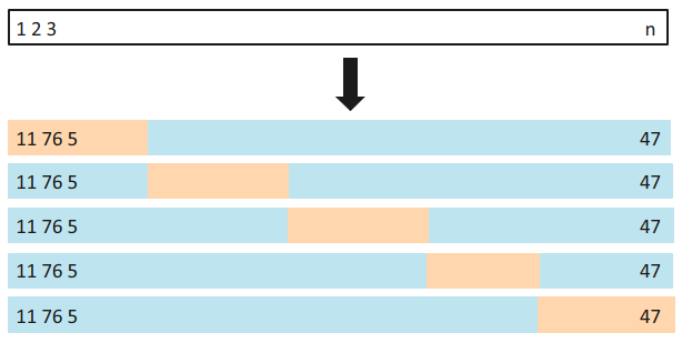
Procedure to estimate prediction error by k-fold (leave-one-out) cross validation
kfold <- function(formula, data, k = 10, criterion){
    n <- nrow(data)
    # Assigning folds
    folds <- sample(rep(1:k, length.out = n))

    # Loop
    eval <- numeric(k)
    for (i in 1:k){
        #splitting the dataset
        train <- data[folds!=i,]
        test  <- data[folds==i,]

        # modelling
        mod     <- lm(formula, data = train)
        pred    <- predict(mod, test)
        y <- all.vars(formula)[1]
        eval[i] <- criterion(test[[y]], pred)
    }

    return(mean(eval))
}kfold(income ~ urban, data = Anscombe, k = 10, Metrics::rmse)
kfold(income ~ urban + young,data = Anscombe, k = 10, Metrics::rmse)## [1] 389.2178
## [1] 432.4814Example/Exercise: Model performance through the years
In this exercise, we explore if a model created in 1952 is still useful for prediction as years go by using some exploratory data analysis. Install and load the package gapminder for this exercise.
Create a new function
lm_validatethat inputs the following:formula: the formula to be usedtrain: training set to be usedtest: test set to be usedcriterion: the evaluation metric function to be used
This should perform the Validation Set Approach for linear regression, but you will have more control which data will be used for training and testing.
Load the dataset
gapminderincluded in the packagegapminder.Filter the dataset to show only values in 1952. Fit a linear regression model that predicts
lifeExpusinglog(gdpPercap)andpop.Using the model in (3) and the function in (1), predict the
lifeExpof each country per year, and show how the RMSE changes through the years. It should look something like this: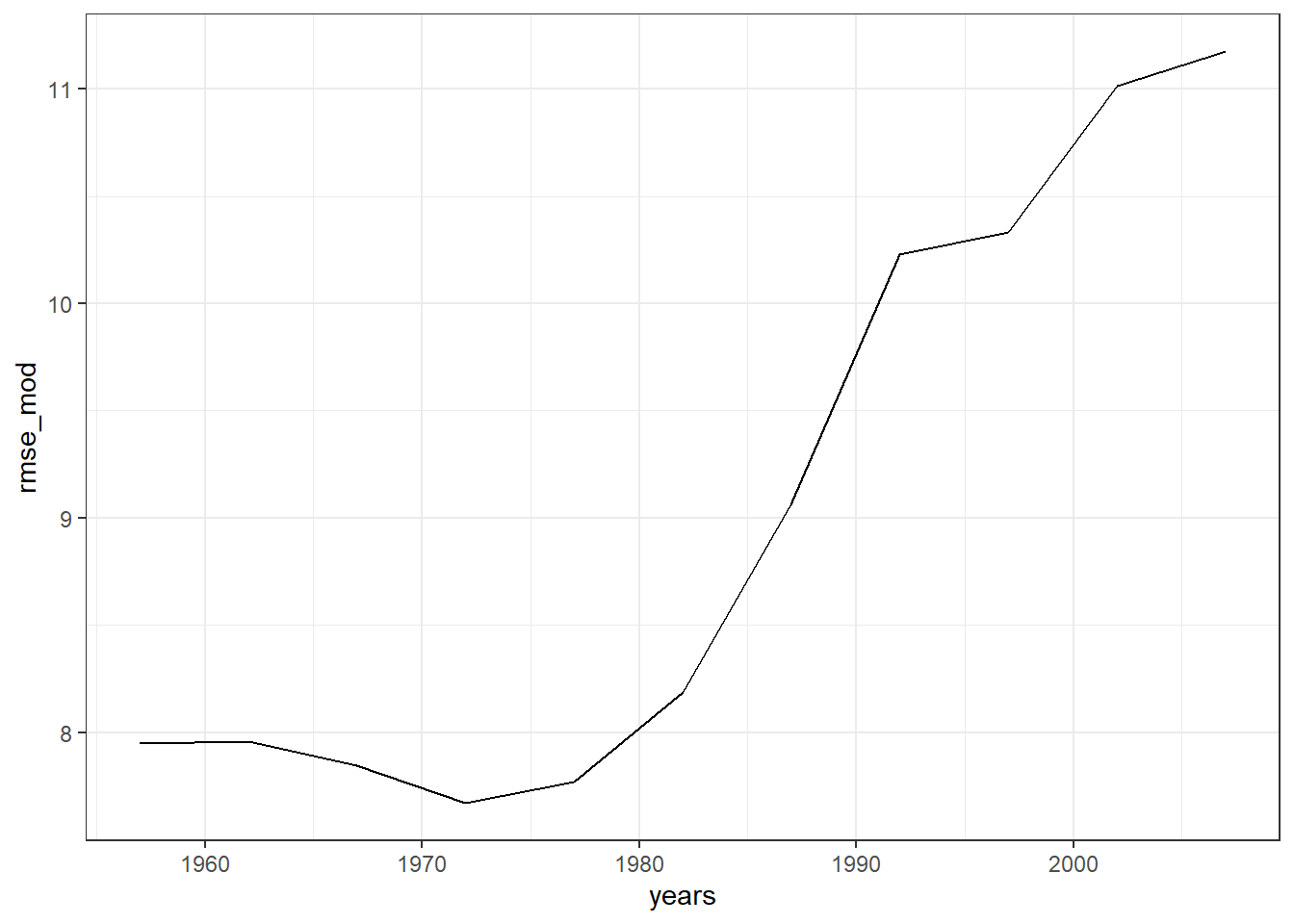
References
Much of the content of this chapter is derived from An Introduction to Statistical Learning with Applications in R (James, Witten, Hastie, & Tibshirani, 2013)
For further reading, you may explore the the cv package by John Fox and Georges Monette:
Introduction to
cvpackage. https://cran.r-project.org/web/packages/cv/vignettes/cv.htmlCross-validating Model Selection. https://cran.r-project.org/web/packages/cv/vignettes/cv-selection.html
axf# Bootstrap in Regression {#bootstrapmodel}
In Chapter 11, we introduced the bootstrap, an exceptionally versatile technique. While it is often applied to estimate the standard deviation of a quantity when direct calculation is difficult or impossible, here we encounter it in a very different role: as a tool to enhance model estimation.
Motivation: Most tests related to model building (e.g. testing the significance of parameters) assumes normality and/or large samples. This is not always the case.
For example, in classical simple linear regression: the Gaussian model assumes that the errors are normally distributed. That is:
\[ y_i = \beta_0+\beta x_i +\varepsilon_i\\ \varepsilon_i \overset{iid}{\sim} N(0,\sigma^2) \]
This further implies the distribution of the OLS estimator has the following distribution:
\[ \hat{\beta} = \frac{\sum(y_i-\bar{y})(x_i-\bar{x})}{\sum(x_i-\bar{x})^2} \sim N\left(\beta,\frac{\sigma^2}{\sum(x_i-\bar{x})^2}\right) \]
And finally,
\[ \frac{\hat{\beta}-\beta}{\widehat{se(\hat{\beta})}} \sim t_{\nu = n-2} \]
where \(\widehat{se(\hat{\beta})}=\sqrt{MSE/\sum(x_i-\bar{x})^2}\)
Inferences about the coefficients \(\beta\) that are based on the T-distribution (e.g. confidence intervals and t-test p-values) will be invalid if the error terms are not normally distributed.
Bootstrap counterparts may be conducted when the data fail to meet these assumptions or data requirement.
Two main resampling schemes in regression will be presented: Case resampling and Model-based resampling. The most basic form of the algorithms are presented here just for the sake of demonstration only.
Concepts here can be used in your final paper, but do not cite this material. You can explore more examples and applications in the book Bootstrap methods and their application by Davison and Hinkley. This is available in the School of Statistics Library.
In the examples, we will use the lmboot package in R.
## Warning: package 'lmboot' was built under R version 4.5.3The bootstrap applications is also extended here to Bagging, which can be used to improve models further, especially if there are many predictors (high-dimensional data).
12.4 Nonparametric Bootstrap Regression
IDEA: Make no parametric assumptions about the model — resample entire data pairs.
Suppose \(y_i\) is the value of the response for the \(i^{th}\) observation, and \(x_{ij}\) is the value of the \(j^{th}\) predictor for the \(i^{th}\) observation. In this example, \(y_i\)s are assumed to be independent such that:
\[ E(y_i|x_i) = \beta_0 + \sum_{j=1}^px_{ij}\beta_j \]
This means the data is cross-sectional, where rows are independent of each other.
Let’s say that the model being fitted is:
\[ y_i= \beta_0 + \sum_{j=1}^p x_{ij}\beta_j+ \varepsilon_i \]
where \(E(\varepsilon_i)=0\), \(Var(\varepsilon_i)=\sigma^2\), \(cov(\varepsilon_i,\varepsilon_j) = 0\).
Do the following to perform inference on \(\beta_j\) via nonparametric bootstrap:
Nonparametric Bootstrap for Regression Coefficient \(\beta_j\)
Input: Dataset
\((y_1,\textbf{x}^T_1),...,(y_n,\textbf{x}^T_n)\)
Output:
Inference on coefficient \(\beta_j\)
Take a simple random sample of size \(n\) with replacement from the data set.
\[ (y_1,\textbf{x}_1^T)^*,...,(y_n,\textbf{x}_n^T)^* \]
This is your bootstrap resample.
Using OLS (or whatever fitting procedure applies), fit a model, and compute the estimates \(\hat{\beta}_j^*\)
Repeat steps 1 and 2 \(B\) times. (\(B\) must be large)
Collect all \(B\) \(\hat{\beta}_j^*\)s and compute measures that apply.
Remarks
The algorithm above is also called “Case-Resampling”
Varying \(X\) but robust
Assumes \((x_j,y_j)\) is sampled from some population. In bootstrapping concept, the bootstrap sample \((x_j,y_j)^*\) is obtained from the joint empirical CDF.
\[ (x_j,y_j)^* \sim EDF((x_1,y_1),...,(x_n,y_n)) \]
Usually no problem in design variation, but can be sometimes awkward in designed experiments and when design is sensitive.
Inference
For POINT estimation
The average of \(\hat{\beta}_j^*\)s is the bootstrap estimate
The estimated standard error is the standard deviation of the \(\hat{\beta}_j^*\)s
Note: the method of averaging the \(\hat{\beta}_j^*\)s is also referred as “Bagging” (See Section 12.6)
For INTERVAL estimation
The simplest approach for constructing a \((1 − \alpha)100\%\) Confidence Interval Estimate is using Percentiles.
\((P_{\alpha/2},P_{1-\alpha/2})\) where \(P_k\) is the \(k^{th}\) quantile.
For interval-based HYPOTHESIS TEST
The usual hypothesis is \(Ho: \beta_j=0\) vs \(Ha:\beta_j\neq0\)
You can use the computed C.I. estimate.
At \(\alpha\) level of significance, reject \(Ho\) when 0 is not in the \((1-\alpha)100\%\) interval estimate.
Example: Suppose you want to fit the following model in the mtcars dataset
\[ \text{mpg} = \beta_0 + \beta_1 \text{wt} + \varepsilon \]
##
## Call:
## lm(formula = mpg ~ wt, data = mtcars)
##
## Coefficients:
## (Intercept)           wt
##      37.285       -5.344
We can use the case-resampling bootstrap method to perform statistical inference on the coefficients \(\beta_0\) and \(\beta_1\).
##     2.5%    97.5%
## 33.04819 42.37606
12.5 Semiparametric Bootstrap Regression
IDEA: Keep the model structure parametric, but resample the residuals nonparametrically.
Note that in the example in Nonparametric Bootstrap Regression, all observations, across columns, are resampled. That assumes that the regressors are also random, which is not the usual case in linear regression.
In the following algorithm, the regressors remain fixed and constant by implementing residual bootstrapping.
Semiparametric Bootstrapping
Input: Dataset
\((y_1,\textbf{x}^T_1),...,(y_n,\textbf{x}^T_n)\)
Output:
Inference on coefficient \(\beta_j\)
Fit the model using the original data to obtain:
the coefficient estimates \(\hat{\beta}_0,\hat{\beta}_1,...,\hat{\beta}_k\)
the fitted values \(\hat{y}_i=\hat{\beta}_0 + \hat{\beta_1}x_{i1} + \cdots + \hat{\beta_k}x_{ik}\)
the residuals \(e_i=y_i-\hat{y}_i\)
From the residuals \((e_1,...,e_n)\), sample with replacement to obtain bootstrap residuals \((e_1^*,e_2^*,...e_n^*)\).
Using the resampled residuals, create a synthetic response variable \(y_i^*=\hat{y}_i+e_i^*\)
Using the synthetic response variable \(y_i^*\), refit the model to obtain bootstrap estimate of the coefficients \(\hat{\beta}_0^*,\hat{\beta}_1^*,\cdots,\hat{\beta}_k^*\)
Repeat 2,3,4 \(B\) times to obtain \(B\) values of \(\hat{\beta}_0^*,\hat{\beta}_1^*,\cdots,\hat{\beta}_k^*\)
Compute measures that apply (e.g. standard error, confidence intervals, etc…)
Interval Estimation and Hypothesis Test follow the same concept.
Remarks
This fixes the design, but not robust to model failure
Instead of assuming that \(x\) and \(y\) has some joint distribution, this properly assumes that the \(x\)s are fixed, and the error term is the one that is sampled from some population.
For this case, we assume that the bootstrapped errors \(\varepsilon^*_j\) can be sampled from the empirical distribution of the residuals.
\[ y_j^*=x_j^T\hat{\beta} + \varepsilon_j^*, \quad \varepsilon_j^*\sim ECDF(e_1-\bar{e}, e_2-\bar{e},...,e_n-\bar{e}) \]
Continuing the example from earlier…
##     2.5%    97.5%
## 33.74770 40.73453
12.6 Bagging Algorithm
Bootstrap aggregating (or bagging) is a useful technique to improve the predictive performance of models, e.g., for additive models with high-dimensional predictors.
The idea is to generate several models via bootstrap and aggregate predicted values via averaging.
Bagging is commonly used to improve tree models or decision trees (such method is called random forest)
It is ideal for minimizing the instability or variance of a model in terms of prediction
The following are some examples of application of bagging in regression.
Algorithm: Basic Bagging for Prediction
Inputs:
The training dataset \((\textbf{y},\textbf{X})\) with \(n\) independent observations.
A fitting procedure \(\mathcal{A}(.)\), such as ordinary least squares
Number of bootstrap replications \(B\)
New dataset \(\textbf{X}_{new}\) that we want to get predictions of \(y\) from.
Output:
- The “bagged” predicted value \(\hat{\textbf{y}}_{bag}\) of the new dataset \(\textbf{X}_{new}\)
Step 1: For \(b\) in \(1\) to \(B\):
Draw a bootstrap sample \((\textbf{y}^*_b,\textbf{X}^*_b)\) of size \(n\) with replacement from \((\textbf{y},\textbf{X})\)
Fit a model using the fitting procedure \(\mathcal{A}\) on the bootstrap sample
\[ \hat{f}_b=\mathcal{A}(\textbf{y}^*_b,\textbf{X}^*_b) \]
Compute predicted value on the new data
\[\widehat{\textbf{y}_b}=\hat{f}_b(\textbf{X}_{new})\]
Step 2: Aggregate the predictions
\[\widehat{\textbf{y}}_{bag}=\frac{1}{B}\sum_{b=1}^B\widehat{\textbf{y}_b}\]
Remarks:
The fitting procedure \(\mathcal{A}\) may correspond to any estimator: parametric, nonparametric, linear, or nonlinear.
Each bootstrap sample produces a different model due to resampling variability.
Bagging reduces variance by averaging predictions across models.
For ordinary least squares, gains are most evident when predictors are highly correlated or the sample size is small.
bagging <- function(train, test, formula, model, B){
    # formula: y~x
    # model: a function that is used to fit a model, such as lm
    y.star <- matrix(nrow = nrow(test), ncol = B)
    n <- nrow(train)
    for(b in 1:B){
        index <- sample(1:n, replace = T)
        train.star <- train[index,]
        mod.star   <- model(formula, data = train.star)
        y.star[,b] <- predict(mod.star, test)
    }
    y.bag <- apply(y.star, 1, mean)
    return(y.bag)
}
You can modify the R code above to accommodate the various extensions of bagging introduced in this book.
Pros and Cons of Bagging
PRO: Bagging induces flexibility in the model
Imagine having a non-linear function formed by aggregating several linear functions with different slopes.
Each base model captures a different linear or local behavior of the data, and their aggregation results in a smooth, flexible function that can approximate complex relationships.
This is advantageous for cases where:
The regression function switches across different regimes or segments (piecewise or overlapping relationships).
The grouping or switching mechanism is hidden or unknown a priori.
CON: The predictive model is hard to interpret.
While bagging improves prediction accuracy, it sacrifices interpretability. Since the final model is an average or majority vote of many base learners, it becomes difficult to trace how each predictor influences the outcome.
Thus, bagging is best suited for applications where:
Prediction accuracy is prioritized over interpretability.
The user is interested in reliable forecasts rather than model explanation.
Examples include financial forecasting, image recognition, and medical diagnostics.
As of now, the basic bagging algorithm is still not that useful.
While bagging can improve predictions for many regression methods, it is particularly useful for “decision trees”, which is not discussed in this course.
Bagging has inspired several useful modifications to its resampling and model-building steps.
Two basic approaches are Random Subsampling and Random Permutations of Predictors.
These techniques are further extended for the computation of Out-of-Bag Errors and Variable Importance Measures.
Random Subsampling
In standard bagging, each bootstrap sample has the same size \(n\) as the original dataset.
Random Subsampling modifies this by taking a smaller sample of size \(m<n\).
That is, instead of resampling \(n\) observations with replacement, we randomly draw \(m\) observations.
Bagging with Random Subsampling
Inputs:
- The training dataset \((\textbf{y},\textbf{X})\)
- Number of bootstrap samples \(B\)
- Subsample size \(m < n\)
- New (unseen) data that contains values of \(\textbf{X}_{new}\) and we want predictions of \(\textbf{y}\).
Outputs:
- The “bagged” predicted value \(\hat{\textbf{y}}_{bag}\) of the new dataset \(\textbf{X}_{new}\)
For \(b=1,2,...,B\):
Draw \(m\) observations from the data (without replacement)
Fit a model \(\hat{f}_b=\mathcal{A}(\textbf{y}^*_b,\textbf{X}_b)\) using the selected \(m\) observations
Use the remaining \(n - m\) observations as the \(b^{th}\) test data
Predict the value of \(\textbf{y}_{new}\) using the new data \(\textbf{X}_{new}\) by plugging in to the fitted model: \(\hat{\textbf{y}}_{b,new}=\hat{f}_b(\textbf{X}_{new})\)
END FOR
COMPUTE “Bagged” predicted value on the new dataset as the average of the predicted values: \(\widehat{\textbf{y}}_{bag}=\frac{1}{B}\sum_{b=1}^B\hat{\textbf{y}}_{b,new}\)
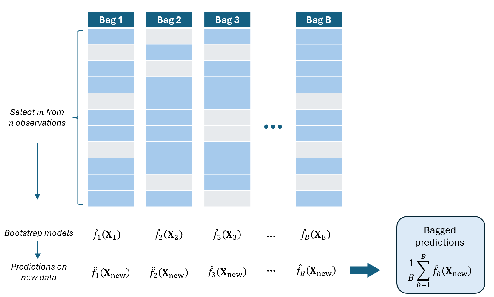
Remarks:
This is almost the same as the basic bootstrap. The only difference is that each bootstrap sample contains only \(m<n\) observations, and elements are obtained without replacement.
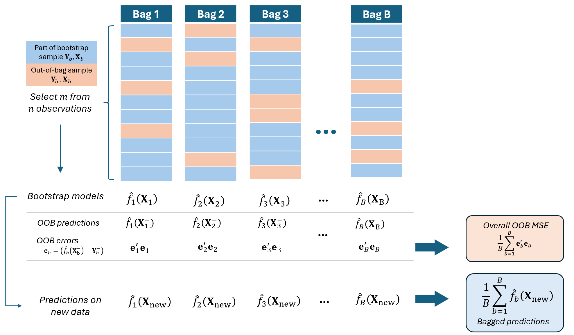
With this approach, we can extend this to obtain “Out-of-Bag Predictions” and estimate “Out-of-Bag Errors” per bootstrap sample.
Out-of-Bag Error Estimation
It turns out that there is a very straightforward way to estimate the test error of a bagged model, without the need to perform cross-validation or the validation set approach.
We can modify the Random Subsampling to enable estimation of the out-of-bag (OOB) error rate for each model:
The remaining \(n-m\) observations not used in training (which we now denote \(\textbf{Y}^-_b, \textbf{X}_b^-\) in this course) will serve as a test dataset for that particular bootstrap sample.
We compute the OOB error as the difference of the out-of-bag observations \(\textbf{Y}^-_b\) and out-of-bag predictions \(\hat{f}_b(\textbf{X}_b^-)\).
The OOB error provides an internal estimate of prediction accuracy without needing a separate validation set.
Hence, random subsampling enhances the efficiency of bagging and supports model evaluation.
This is like inserting a Train-and-Test Validation inside the bagging algorithm.
Random Permutations of Predictors
While Bagging focuses on resampling data, we can introduce additional randomness by randomly selecting or permuting predictors when training each model.
In this approach, you create many models where some models in the ensemble do not contain some predictors. This creates diversity among the models and enhances ensemble performance.
It appeals to relationships where the set of significant predictors vary across different “groups” or “types” of observation.
Bagging with Random Permutations of Predictors
Inputs:
- The training dataset \((\textbf{y},\textbf{X})\)
- Set of \(p\) predictors \(\{X_1, X_2, …, X_p\}\)
- Number of bootstrap samples \(B\)
- Number of predictors to sample per model, \(q < p\)
- New (unseen) data that contains values of \(\textbf{X}_{new}\) and we want predictions of \(\textbf{y}\).
Outputs:
- The “bagged” predicted value \(\hat{\textbf{y}}_{bag}\) of the new dataset \(\textbf{X}_{new}\)
FOR \(b\) in \(1\) to \(B\) DO:
Randomly select \(q\) predictors from \(X_1,...,X_p\).
Fit a model \(\hat{f}_b(\textbf{X})\) using only the selected \(q\) predictors.
Predict the value of \(\textbf{y}_{new}\) using the new data \(\textbf{X}_{new}\) by plugging in to the fitted model: \(\hat{\textbf{y}}_{b,new}=\hat{f}_b(\textbf{X}_{new})\)
END LOOP
COMPUTE “Bagged” predicted value on the new dataset as the average of the predicted values: \(\widehat{\textbf{y}}_{bag}=\frac{1}{B}\sum_{b=1}^B\hat{\textbf{y}}_{b,new}\)
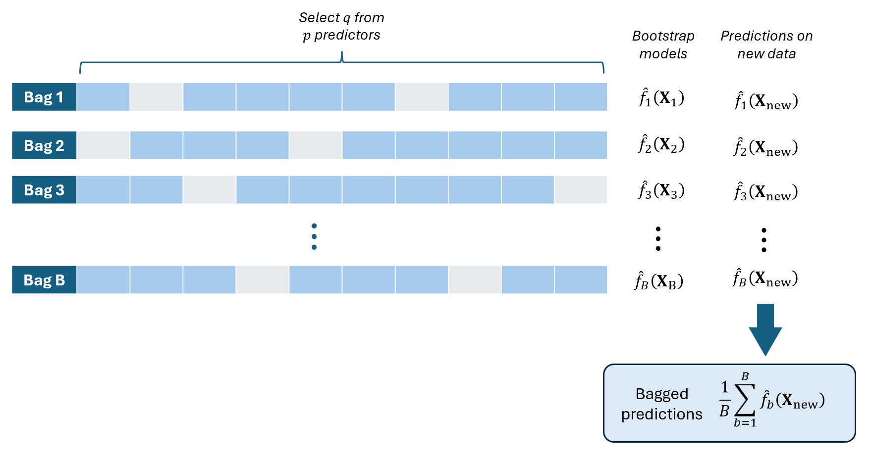
This is especially useful if the number of predictors in your dataset is very high compared to the number of observations (\(p>>n\)). In each bootstrap model, use \(q\leq n\).
Variable Importance Measures
As we have discussed, bagging may improve the prediction accuracy, but the resulting model may be difficult to interpret.
This last method combines the random permutations approach with bagging with OOB error estimation to allow us to evaluate the impact of a variable in the bagged predictive model for a new angle of interpretability.
To compute this, each bootstrap model should be obtained from bootstrap sample \(m<n\) as well, and the OOB prediction error from the test dataset containing \(n-m\) observations must be obtained.
The impact score is usually computed as the difference of the OOB prediction error of models that include the variable from those that do not include the variable.
\[ \text{Impact Score of Variable } X_j = \\mean(\text{Error of Models without } X_j)- mean(\text{Error of Models with } X_j) \]
High impact score implies that the model will perform poorly if the variable \(X_j\) is removed from the model.
Suggestions for Research using Bagging
explore bagging algorithm for a real predictive modeling task. (e.g. improve a linear model via bagging)
bagging algorithm for modeling high dimensional data (i.e. p >> n). Hence, only a subset of variables can be considered at a time.
design a strategic randomization method and/or aggregation strategy for Bagging a certain model.
explore the impact score as a tool for variable selection.
References
Outline and some content of this chapter are derived from handouts of Asst. Prof. Supranes of UP School of Statistics, but here are the main references:
Davison, A. C., & Hinkley, D. V. (1997). Bootstrap Methods and their Application. In Cambridge University Press eBooks. https://doi.org/10.1017/cbo9780511802843
James, G., Witten, D., Hastie, T., & Tibshirani, R. (2018). An Introduction to Statistical Learning: with Applications in R. https://doi.org/10.25334/q4ht55